On this page
In recent times, we’ve heard a lot about these Large Language Models which are able to endlessly generate text, images, video, etc. We often take these Machine Learning models for granted, but there is a distinction between these type of models which generate output vs. those which predict an output. Unlike traditional predictive models, which focus on making predictions or classifications based on existing data, generative models aim to generate new data that mimics the characteristics of the training dataset. This distinction is pivotal, as it opens up a realm of possibilities where machines can not only understand and analyze data but also contribute creatively by producing novel data.
Understanding Generative Models
Generative models are a class of machine learning models that learn the underlying distribution of the training data and can generate new data points that follow this learned distribution. These models can create images, music, text, and even complex structures like 3D objects. The essence of generative models lies in their ability to capture the data distribution and use it to generate new samples that are statistically similar to the original dataset.
Examples of Generative Models
- Gaussian Mixture Models (GMMs): These are probabilistic models that assume all the data points are generated from a mixture of several Gaussian distributions with unknown parameters. GMMs are often used for clustering and density estimation.
- Variational Autoencoders (VAEs): These are deep learning models that encode input data into a latent space and then decode it to reconstruct the original data. VAEs are used for generating new data by sampling from the latent space.
- Generative Adversarial Networks (GANs): GANs are a type of generative model that involves two neural networks — the Generator and the Discriminator — competing against each other to create realistic data. This architecture is particularly effective in generating high-quality images and other types of data.
Non-Generative Models (Predictive Models)
In contrast to generative models, non-generative models, or predictive models, focus on predicting outcomes based on input data. These models do not generate new data but instead learn to map input data to specific outputs. Predictive models are widely used for tasks such as classification, regression, and time-series forecasting.
Examples of Predictive Models
- Linear Regression: This is a fundamental predictive model that estimates the relationship between a dependent variable and one or more independent variables. It is used for predicting numerical outcomes.
- Support Vector Machines (SVMs): These are supervised learning models used for classification and regression tasks. SVMs work by finding the hyperplane that best separates the data into different classes.
- Neural Networks: These models consist of interconnected layers of neurons that learn to map input data to output predictions. They are used for a variety of tasks, including image recognition, language processing, and more.
Now that we have made this very important distinction between generative models vs. predictive models, let’s jump into understanding Generative Adversarial Networks. A generative adversarial network (GAN) is a deep learning architecture. It trains two neural networks to compete against each other to generate more authentic new data from a given training dataset.
For instance, you can generate new images from an existing image database or original music from a database of songs. A GAN is called adversarial because it trains two different networks and pits them against each other. One network generates new data by taking an input data sample and modifying it as much as possible. The other network tries to predict whether the generated data output belongs in the original dataset. In other words, the predicting network determines whether the generated data is fake or real. The system generates newer, improved versions of fake data values until the predicting network can no longer distinguish fake from original.
breaking down GANs
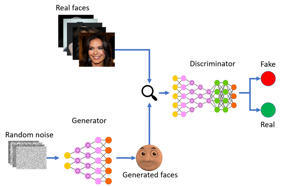
Before going head first into implementating a GAN from scratch, let’s take a step back and understand the mathematical and theoretical aspects of how a Generative Adversarial Network works. GANs are a type of deep learning architecture; at a high level, GANs train 2 neural networks against each other and they basically compete against one another — they compete with each other to improve their performance continuously. Here is a quick diagram which shows how everything works together:

You may notice some terminology in the diagram that we haven’t touched on, but to break it down, each of the 2 neural networks have a name. The neural network that produces new data is called the generator. The neural network that distinguishes whether or not it belongs in the original dataset is called the discriminator. Now that we have a rough understanding of how these things work, let’s jump into the specifics of both the generator and discriminator.
understanding the generator
Input to the Generator
The generator takes as input a random noise vector, often sampled from a simple distribution such as a uniform or Gaussian distribution. This vector is typically of lower dimensionality compared to the real data distribution. The noise vector serves as a source of randomness, allowing the generator to produce a wide variety of outputs.
Architecture of the Generator
The architecture of the generator can vary, but it generally consists of a series of layers that progressively transform the input noise vector into a structured data format. Here’s a breakdown of a typical generator architecture:

- Dense Layers: The noise vector is first passed through one or more fully connected (dense) layers. These layers help to scale up the low-dimensional noise vector into a higher-dimensional feature space. Example: For an input noise vector zzz of dimension 100, the first dense layer might have 1024 units, transforming the 100-dimensional vector into a 1024-dimensional one.
- Batch Normalization: To stabilize the training and improve the learning process, batch normalization is often applied after the dense layers. This normalizes the output of the previous layer, maintaining the mean output close to 0 and the output standard deviation close to 1. Effect: Batch normalization helps in reducing the internal covariate shift and accelerates the training process.
- Activation Functions: Non-linear activation functions such as ReLU (Rectified Linear Unit) or Leaky ReLU are applied to introduce non-linearity into the model, allowing it to learn more complex patterns. Example: After the dense layers and batch normalization, a ReLU activation function might be applied to the output.
- Transpose Convolutional Layers: To transform the high-dimensional feature space into the desired output shape (e.g., an image), transpose convolutional layers (also known as deconvolutional layers) are used. These layers perform upsampling, effectively reversing the operation of convolutional layers and increasing the spatial dimensions of the data. Example: A 256-dimensional feature map might be upsampled through several transpose convolutional layers to create a 64x64x3 image.
- Output Layer: The final layer of the generator uses a suitable activation function to produce the output in the required format. For example, in image generation, a tanh activation function might be used to scale the pixel values to the range [-1, 1]. Example: The output layer could be a transpose convolutional layer followed by a tanh activation function to generate the final image.
Generator Loss Function
The generator’s goal is to produce data that the discriminator cannot distinguish from real data. Therefore, the loss function for the generator is based on the performance of the discriminator. Specifically, the generator aims to maximize the discriminator’s error rate.
Mathematically, the generator’s loss can be represented as:

Here:
- z is the input noise vector.
- G(z) is the output of the generator.
- D(G(z)) is the discriminator’s probability that the generated data is real.
- E denotes the expected value.
In practice, this loss is minimized using gradient descent. The generator receives gradients from the discriminator and updates its weights to improve its output quality. Now that we have a rough understanding of how the generator is structured, let’s implement this in python! I’m not going to bother boring you guys with the implementation of each layer i.e dense, convolutional, batch normalization, etc. If you want the exact implementation of what each layer would look like, feel free to check out my github repository here, it has all the layers implemented from scratch :)
def build_generator(noise_dim):
    model = models.Sequential()

    # Dense layer to scale up the noise vector
    model.add(layers.Dense(7 * 7 * 256, use_bias=False, input_shape=(noise_dim,)))
    model.add(layers.BatchNormalization())
    model.add(layers.ReLU())

    # Reshape to start the convolutional stack
    model.add(layers.Reshape((7, 7, 256)))
    assert model.output_shape == (None, 7, 7, 256)

    # Transpose Convolutional Layer 1
    model.add(layers.Conv2DTranspose(128, (5, 5), strides=(1, 1), padding='same', use_bias=False))
    assert model.output_shape == (None, 7, 7, 128)
    model.add(layers.BatchNormalization())
    model.add(layers.ReLU())

    # Transpose Convolutional Layer 2
    model.add(layers.Conv2DTranspose(64, (5, 5), strides=(2, 2), padding='same', use_bias=False))
    assert model.output_shape == (None, 14, 14, 64)
    model.add(layers.BatchNormalization())
    model.add(layers.ReLU())

    # Transpose Convolutional Layer 3
    model.add(layers.Conv2DTranspose(1, (5, 5), strides=(2, 2), padding='same', use_bias=False, activation='tanh'))
    assert model.output_shape == (None, 28, 28, 1)

return modelSome of this code may look foreign so let’s dive into what each layer in the model is doing. We start off by creating a dense layer. The first layer in the generator is a dense (fully connected) layer that scales up the noise vector from a lower-dimensional space to a higher-dimensional space.
- Implementation: The layer is defined with
7 * 7 * 256units anduse_bias=False. Theinput_shapeis specified as(noise_dim,), wherenoise_dimis the dimensionality of the input noise vector. - Effect: This transformation is crucial as it prepares the noise vector for subsequent convolutional layers by increasing its dimensionality and allowing it to be reshaped into a multi-channel feature map.
Next up, we have a batch normalization layer. We apply batch normalization right after the input is passed through the dense layer.
- Implementation: The
BatchNormalizationlayer normalizes the output of the dense layer so that its mean output is close to 0 and its standard deviation is close to 1. - Effect: This normalization helps in stabilizing and accelerating the training process by reducing internal covariate shift.
- ReLU Activation:
- Purpose: A ReLU (Rectified Linear Unit) activation function is applied to introduce non-linearity into the model.
- Implementation: The
ReLUlayer replaces all negative values in the feature map with zeros, while positive values remain unchanged. - Effect: This non-linearity allows the model to learn more complex patterns and relationships in the data.
Reshape Layer:
- Purpose: The reshape layer changes the shape of the output from the previous dense layer into a 3D tensor suitable for convolutional operations.
- Implementation: The
Reshapelayer transforms the flat vector of shape(7 * 7 * 256,)into a 3D tensor of shape(7, 7, 256). - Effect: This step prepares the data for upsampling through transpose convolutional layers, mimicking the initial feature maps of an image.
Transpose Convolutional Layer 1:
- Purpose: This layer performs upsampling to increase the spatial dimensions of the feature map.
- Implementation: A
Conv2DTransposelayer is used with 128 filters, a kernel size of(5, 5), strides of(1, 1), andpadding='same'.use_bias=Falseis specified to avoid bias addition. - Effect: The feature map size remains
(7, 7)due to the stride of 1, but the depth changes from 256 to 128, preparing the feature map for further upsampling.
Batch Normalization and ReLU:
- Purpose: These layers repeat the normalization and non-linearity steps to stabilize training and introduce complexity.
- Implementation: The
BatchNormalizationandReLUlayers are applied sequentially. - Effect: They normalize the outputs and introduce non-linearity, respectively, which helps in learning more complex patterns.
Transpose Convolutional Layer 2:
- Purpose: This layer further upsamples the feature map.
- Implementation: Another
Conv2DTransposelayer is added with 64 filters, a kernel size of(5, 5), strides of(2, 2), andpadding='same'. - Effect: The spatial dimensions of the feature map are increased from
(7, 7)to(14, 14)due to the stride of 2, while the depth changes from 128 to 64.
Batch Normalization and ReLU:
- Purpose: These layers again normalize the outputs and introduce non-linearity.
- Implementation: The
BatchNormalizationandReLUlayers are applied sequentially. - Effect: They help in stabilizing the training and learning complex patterns.
Transpose Convolutional Layer 3:
- Purpose: The final transpose convolutional layer upsamples the feature map to the desired output dimensions.
- Implementation: A
Conv2DTransposelayer with 1 filter, a kernel size of(5, 5), strides of(2, 2),padding='same', andactivation='tanh'is used. - Effect: This layer increases the spatial dimensions from
(14, 14)to(28, 28), which is typically the size of the output image (e.g., in MNIST). Thetanhactivation scales the pixel values to the range[-1, 1], suitable for image data.
Overall, the generator architecture ensures that the generator transforms a simple noise vector into a high-dimensional, realistic image by progressively upsampling and refining the feature maps through a series of layers. Now that we have a solid understanding of the generator, let’s jump into understanding the discriminator!
The Discriminator
The discriminator in a Generative Adversarial Network (GAN) is a neural network that acts as a binary classifier, distinguishing between real data samples and those generated by the generator. Its primary function is to evaluate the authenticity of the data samples it receives, providing feedback to both itself and the generator during the training process. The discriminator’s goal is to correctly classify real data as real and generated (fake) data as fake.
How the Discriminator Works
The discriminator receives both real data from the training dataset and fake data from the generator. It then processes these inputs through a series of layers to produce a probability score, typically between 0 and 1, where 1 indicates a high likelihood that the input is real, and 0 indicates a high likelihood that the input is fake. During training, the discriminator is updated to improve its classification accuracy, while the generator is updated to produce data that can fool the discriminator into classifying fake data as real.
Architecture of the Discriminator
The architecture of the discriminator typically involves several convolutional layers followed by dense layers. Here is a detailed breakdown of a typical discriminator architecture:
- Input Layer:
- The discriminator takes as input an image (or other data types in other applications). For simplicity, let’s consider grayscale images of size 28x28x1, as used in the MNIST dataset.
Convolutional Layer 1:
- Purpose: Extract low-level features from the input image.
- Implementation: A
Conv2Dlayer with 64 filters, a kernel size of(5, 5), strides of(2, 2), andsamepadding. The convolution operation scans the image and applies filters to detect edges, textures, and other basic patterns. - Activation: A Leaky ReLU activation function is applied to introduce non-linearity. Leaky ReLU allows a small gradient when the unit is not active, preventing dead neurons.
- Effect: This layer reduces the spatial dimensions of the image from 28x28 to 14x14 and increases the depth to 64, highlighting the important features in the image.
Dropout Layer:
- Purpose: Prevent overfitting by randomly setting a fraction of input units to zero during training.
- Implementation: A
Dropoutlayer with a rate of 0.3. - Effect: This regularizes the model and improves its generalization to unseen data.
Convolutional Layer 2:
- Purpose: Extract higher-level features from the feature map produced by the first convolutional layer.
- Implementation: A
Conv2Dlayer with 128 filters, a kernel size of(5, 5), strides of(2, 2), andsamepadding. - Activation: Another Leaky ReLU activation function is applied.
- Effect: This layer reduces the spatial dimensions further from 14x14 to 7x7 and increases the depth to 128, capturing more complex patterns in the image.
Dropout Layer:
- Purpose: Further regularization to prevent overfitting.
- Implementation: A
Dropoutlayer with a rate of 0.3. - Effect: Enhances the model’s ability to generalize by randomly dropping units during training.
Flatten Layer:
- Purpose: Convert the 3D feature map into a 1D feature vector to prepare it for the dense layers.
- Implementation: A
Flattenlayer. - Effect: The output shape is transformed from (7, 7, 128) to (6272,).
Dense Layer:
- Purpose: Classify the input based on the extracted features.
- Implementation: A
Denselayer with a single unit. - Activation: No activation function is applied in this layer as we directly use the raw output for the final classification.
- Effect: This layer produces a single scalar value representing the probability that the input image is real.
Activation Function:
- Purpose: Convert the raw output score to a probability.
- Implementation: A sigmoid activation function is applied to the output of the dense layer.
- Effect: The sigmoid function maps the output to a value between 0 and 1, representing the probability that the input is real.
Discriminator Loss Function
The discriminator’s loss function consists of two parts:
- Real Loss: The loss when the discriminator correctly identifies real images as real.
- Fake Loss: The loss when the discriminator correctly identifies generated images (fake images) as fake.
The overall loss for the discriminator is the sum of these two losses.
Binary Cross-Entropy Loss

Binary cross-entropy loss is commonly used for binary classification tasks. For the discriminator in a GAN, the binary cross-entropy loss for real and fake images can be computed as follows:
- Real Loss: Calculated as the binary cross-entropy between the discriminator’s predictions for real images and the target labels (which are 1s, indicating real).
- Fake Loss: Calculated as the binary cross-entropy between the discriminator’s predictions for generated (fake) images and the target labels (which are 0s, indicating fake).
Here’s the implementation of the discriminator based on the architecture described:
def build_discriminator(input_shape=(28, 28, 1)):
    model = models.Sequential()

    # Convolutional Layer 1
    model.add(layers.Conv2D(64, (5, 5), strides=(2, 2), padding='same', input_shape=input_shape))
    model.add(layers.LeakyReLU())
    model.add(layers.Dropout(0.3))

    # Convolutional Layer 2
    model.add(layers.Conv2D(128, (5, 5), strides=(2, 2), padding='same'))
    model.add(layers.LeakyReLU())
    model.add(layers.Dropout(0.3))

    # Flatten and Dense Layer
    model.add(layers.Flatten())
    model.add(layers.Dense(1))

    return model


discriminator = build_discriminator()Training the GAN
Now that we have an understanding of how the 2 main components of the GAN works, let’s put this together and build a GAN in python! Feel free to use the code below! On the github, there’s some code that I made to run it on the MNIST dataset, feel free to try it out!
class GAN(tf.keras.Model):
    def __init__(self, generator, discriminator):
        super(GAN, self).__init__()
        self.generator = generator
        self.discriminator = discriminator

    def compile(self, g_optimizer, d_optimizer, loss_fn):
        super(GAN, self).compile()
        self.g_optimizer = g_optimizer
        self.d_optimizer = d_optimizer
        self.loss_fn = loss_fn


    def train_step(self, real_images):
        batch_size = tf.shape(real_images)[0]
        noise = tf.random.normal([batch_size, self.generator.input_shape[-1]])

        # Train the discriminator
        with tf.GradientTape() as d_tape:
            generated_images = self.generator(noise, training=True)
            real_output = self.discriminator(real_images, training=True)
            fake_output = self.discriminator(generated_images, training=True)
            d_loss_real = self.loss_fn(tf.ones_like(real_output), real_output)
            d_loss_fake = self.loss_fn(tf.zeros_like(fake_output), fake_output)
            d_loss = d_loss_real + d_loss_fake


        d_gradients = d_tape.gradient(d_loss, self.discriminator.trainable_variables)
        self.d_optimizer.apply_gradients(zip(d_gradients, self.discriminator.trainable_variables))

        # Train the generator
        with tf.GradientTape() as g_tape:
            generated_images = self.generator(noise, training=True)
            fake_output = self.discriminator(generated_images, training=True)
            g_loss = self.loss_fn(tf.ones_like(fake_output), fake_output)


        g_gradients = g_tape.gradient(g_loss, self.generator.trainable_variables)
        self.g_optimizer.apply_gradients(zip(g_gradients, self.generator.trainable_variables))


return {"d_loss": d_loss, "g_loss": g_loss}Training Process
The training process of the generator is tightly coupled with that of the discriminator. During training, the following steps are typically repeated iteratively:
- Generate Fake Data: The generator takes random noise vectors as input and produces fake data.
- Train Discriminator: The discriminator is trained on both real data and the fake data generated by the generator. It updates its weights to better distinguish between real and fake data.
- Train Generator: The generator is trained to maximize the discriminator’s error on the fake data, effectively learning to generate more realistic data over time.
The iterative training continues until a desired level of performance is achieved, where the generator produces high-quality data that the discriminator cannot easily distinguish from real data.
That marks the end of understanding GANs from a theoretical level and using them on a sample dataset. I hope that reading this article added value to you and provided a clear understanding of how to use a GAN and the inner workings of the generator & discriminator architecture. That was a long article, but if you’ve read till the end, thank you so much for taking time to read my article and I hope you walked away with more knowledge than you came in with :)
If you have any questions regarding this article or just want to connect, you can find me on LinkedIn or my personal website :)